A Gentle Introduction of NTT - Part III: The Kyber Trick

In the previous post, we have seen that NTT is a special way of evaluating a polynomial (i.e. converting a polynomial from coefficient form to evaluation form) such that the evaluation points are all the $d$-th roots of unity. We then examined a few efficient ways (recursive and iterative) to implement NTT and iNTT routines. Lastly we learned that by carefully picking the right twiddle factors (generators) as roots of the polynomial modulus, we can perform modular polynomial multiplication in NTT form in the same degree as the multiplicand (without the need to extend the degree and perform additional reduction).

Putting everything we’ve learned so far, we can put together an efficient algorithm for multiply polynomials in a ring in $O(n \log{n})$ time. The recipe is as simple as:

1. Perform NTT on polynomial $P, Q$ with the roots of the polynomial modulus $\phi$ as twiddle factors and obtain $\hat{P}, \hat{Q}$. Note that this requires the modulus to have a special structure such that there exists a generator that generates all of its roots.

2. Perform coordinate-wise multiplication on $\hat{P}, \hat{Q}$ and obtain $\hat{R}$.

3. Perform Inverse NTT on $\hat{R}$ and recover the final multiplication result $R = P \times Q$.

NWC, revisited

From the previous post, we also saw that there are two commonly used cyclotomic polynomial moduli in NTT - $x^d - 1$ that corresponds to circular convolution (CC), and $x^d + 1$ that corresponds to negative-wrapped convolution (NWC).

In this post, we will continue our discussion on the Negative-Wrapped Convolution (NWC).

One of the key speed-up for polynomial multiplication brought by NTT is that, if the evaluation points happen to be the roots of the polynomial modulus (in our case, $x^d \pm 1$), then the multiplication result is automatically reduced to the target degree, and hence we don’t have to double the length/degree of the polynomial we are multiplying to preserve the higher degree coefficients for the reduction.

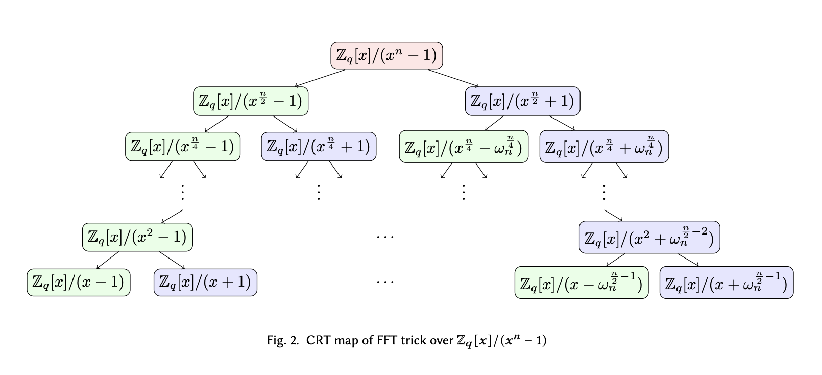
In the case of $x^d - 1$, we found out that the distinct powers of a $d$-th primitive root of unity $\omega_d^i$ (or alternatively, the set of field elements generated by the generator $\omega_d$) also happens to be all the roots for the polynomial modulus:

How we obtained this result is through recursively splitting the $x^d - 1$ term, and applying the fact that $\omega_d^\frac{d}{2} \equiv -1$ to convert the addition term after the split back into a subtraction term so we can split further. For example, $x^\frac{d}{2} + 1 \rightarrow x^\frac{d}{2} - \omega_d^\frac{d}{2}$. We can split totally $\log{d}$ times and end up with $d$ unsplittable degree-1 terms in which we can easily extract the roots of the original polynomial from. As seen from the last post, we can represent the splitting operation as a binary tree shown below (ignoring the $\mathbb{Z}_q[x]/$ part of the expression and $n = d$):

Now moving to the case of NWC. We perform the same kind of binary split and result in the following tree ($\omega_d = \phi_{2d}^2$):

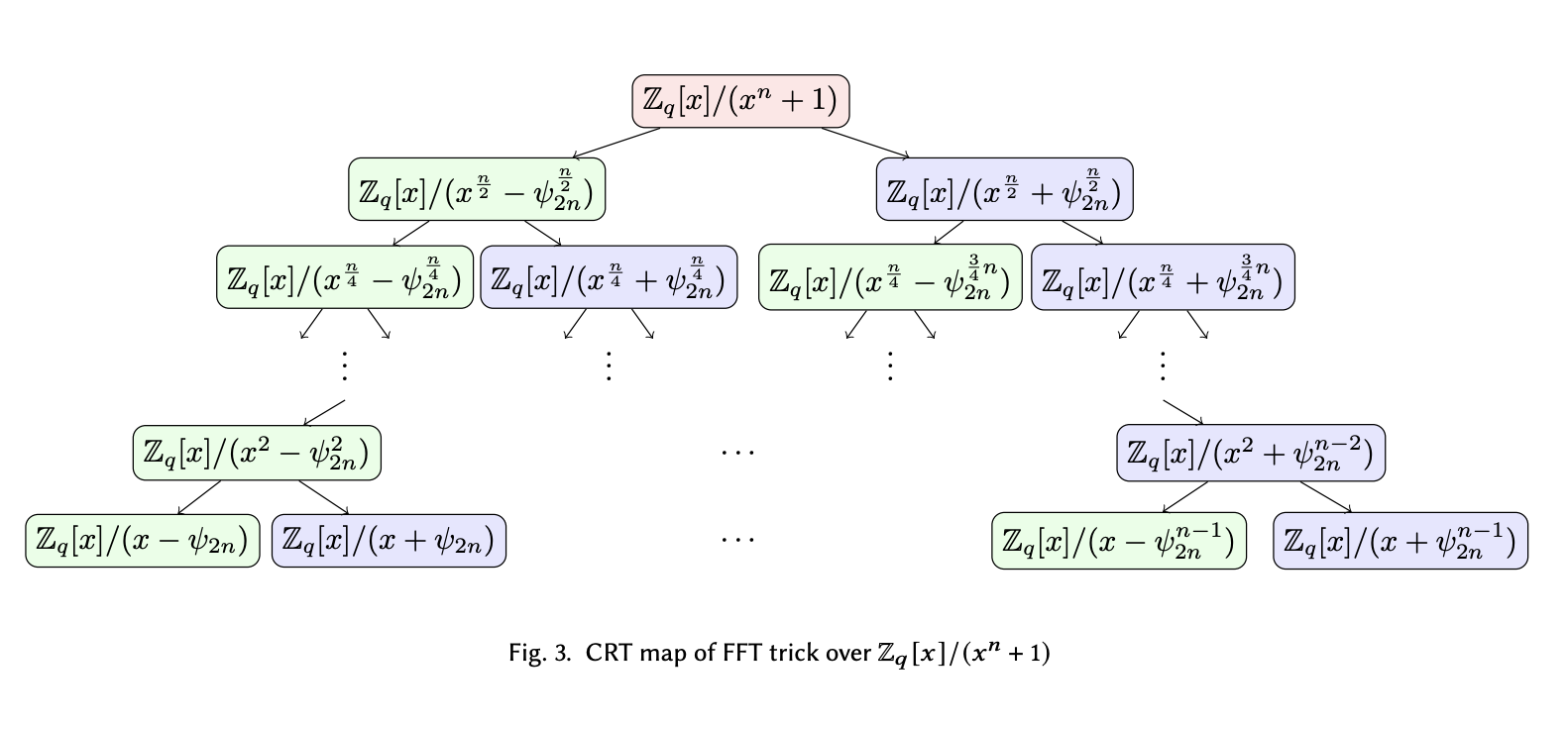
One problem with the same approach that we pointed out last time is that, starting from the second layer from the top of the tree, the degree of the $\omega$ term on the right is always one half of the degree of the $x$ term on the left. This means that we will run out of $\omega$ terms to split with before we have fully splitted the $x$ terms down to degree-1. As seen on the second layer from the bottom of the tree, $x^2 - \omega_d$ cannot be broken down further, until the point we introduced a finer generator $\phi_{2d}$ which can help us split $\omega_d$ one more time. With $\phi_{2d}$ as the new $2d$-th root of unity, we found the roots of the original polynomial, which are distinct odd powers of the new generator.

Performance Penalty

The roots for the NWC case indeed work for our polynomial multiplication task. However, we are putting more constraints on the properties of the underlying field $\mathbb{Z}_q$: to make sure everything is well-defined, we need to make sure that the $2d$-th primitive root of unity actually exists in the field. So far, we’ve kind of taken it for granted assuming that $\omega_d$ exists in $\mathbb{Z}_q$. However, it doesn’t necessarily mean that we can also find the $2d$-th one.

For example, the field $q$ used in Kyber is 3329, in which number 17 is a qualifying 256-th primitive root of unity (one can easily check that $17^{256} \equiv 1 \text{ mod } 3329, 17^{128} \equiv -1 \text{ mod } 3329$). Sadly, the 512-th one doesn’t exist. If we happen to work in the NWC polynomial modulus, we can only perform degree-128 polynomial multiplications! If we really want to do degree-256 polynomial multiplications, we will have to make the underlying field much larger. The smallest field that gives us a 512-th primitive root of unity is 12289 (with number 3 as an example generator such that $3^{512} \equiv 1 \text{ mod } 12289, 3^{256} \equiv -1 \text{ mod } 12289$), which is the field used in another key encapsulation system called NewHope.

The bump from 3329 to 12289 to accommodate degree-256 polynomial multiplication can cause potential performance impacts. Sice $3329 \approx 2^{11.7}$ and $12289 \approx 2^{13.6}$, we are looking at a 2-bit increase of the representation of the underlying field size, and a 4x timing/memory degrade if we have to pre-compute things in the field and store them offline.

This naturally brings us to the next big question: Can we do better?

Just split something else

The short answer to the question is: Yes, but not without paying some price.

To avoid paying the extra cost in the field, we will just have to figure out a way to work without the assumption of the existence of $\phi_{2d}$. Now we are back in the binary split tree, and stuck at the layer where we are left with a term that looks like $x^2 - \omega_d$.

To get us unblocked, here’s some life advice: If you cannot have what you want, you should want what you can have.

Halving the dimensions

If the best thing we can have is the existence of a primitive $d$-th root of unity $\omega_d$, then using the same NTT with NWC approach, we will see what we can do with it.

Here is a simple idea: let’s constrain everything we work with to only be $\frac{d}{2}$-degree polynomials, and define the NTT operation on them. Because we only have $\frac{d}{2}$ coefficients, we only need half the evaluations. Since we know $\omega_d$ already, we can easily set $\omega_\frac{d}{2} = \omega_d^2$ to be the new $\frac{d}{2}$-th primitive root of unity, and conversely $\phi_d = \omega_d$. We call this operation the half-NTT, as it operates on input vectors half the size of our intended targets.

Now, applying everything we’ve known previously, we can now do degree-$\frac{d}{2}$ polynomial multiplication coordinate-wise without reductions with $x^\frac{d}{2} + 1$ as the polynomial modulus. Effectively, we halve the size of $d$ to make sure the $2d$-th primitive root of unity exists in the field.

Split the target polynomial

How can we make use of the newly defined half-NTT procedures? Here is another intuition: can we break down polynomial multiplications in degree-$d$ into several polynomial multiplications in degree-$\frac{d}{2}$?

Take a degree-4 polynomial $P$ as an example:

We see that we can reorder the terms and factor the common parts and essentially interpret a polynomial as a combination of a polynomial with only even coefficients and a polynomial with only odd coefficients. This is very similar to the FFT-like recurrence relation trick that we did in the previous post to speed up NTT.

The important part is that, since each of the smaller polynomials $P^\text{even}, P^\text{odd}$ has only half of the coefficients of $P$, we know that it has degree $\frac{d}{2}$. Therefore, our half-NTT procedure would work on them!

Let’s now set up the half-NTT procedure programmatically. We first import the efficient iterative NTT/iNTT implementations from the previous post. We also directly work in the Kyber field $q = 3329$ to demonstrate how it works IRL.

# We use the Kyber modulus
MODULUS = 3329
GEN = 17
GEN_INV = pow(GEN, -1, MODULUS)
# 17 is a primitive 256-th root of unity of modulus 3329.
# Therefore, we will be working with polynomials with length 256 (degree 255).
assert pow(GEN, 256, MODULUS) == 1
assert pow(GEN, 128, MODULUS) != 1

# We import the NTT routines from last post.
# BEGIN: REFERENCE
import math

def brv(x, n):
  """ Reverses a n-bit number """
  return int(''.join(reversed(bin(x)[2:].zfill(n))), 2)

def ntt_iter(a, gen=GEN, modulus=MODULUS):
  deg_d = len(a)

  # Start with stride = 1.
  stride = 1

  # Shuffle the input array in bit-reversal order.
  nbits = int(math.log2(deg_d))
  res = [a[brv(i, nbits)] for i in range(deg_d)]

  # Pre-compute the generators used in different stages of the recursion.
  gens = [pow(gen, pow(2, i), modulus) for i in range(nbits)]
  # The first layer uses the lowest (2nd) root of unity, hence the last one.
  gen_ptr = len(gens) - 1

  # Iterate until the last layer.
  while stride < deg_d:
    # For each stride, iterate over all N//(stride*2) slices.
    for start in range(0, deg_d, stride * 2):
      # For each pair of the CT butterfly operation.
      for i in range(start, start + stride):
        # Compute the omega multiplier. Here j = i - start.
        zp = pow(gens[gen_ptr], i - start, modulus)

        # Cooley-Tukey butterfly.
        a = res[i]
        b = res[i+stride]
        res[i] = (a + zp * b) % modulus
        res[i+stride] = (a - zp * b) % modulus

    # Grow the stride.
    stride <<= 1
    # Move to the next root of unity.
    gen_ptr -= 1

  return res

def intt_iter(a, gen=GEN, modulus=MODULUS):
  deg_d = len(a)

  # Start with stride = N/2.
  stride = deg_d // 2

  # Shuffle the input array in bit-reversal order.
  nbits = int(math.log2(deg_d))
  res = a[:]

  # Pre-compute the inverse generators used in different stages of the recursion.
  gen = pow(gen, -1, modulus)
  gens = [pow(gen, pow(2, i), modulus) for i in range(nbits)]
  # The first layer uses the highest (d-th) root of unity, hence the first one.
  gen_ptr = 0

  # Iterate until the last layer.
  while stride > 0:
    # For each stride, iterate over all N//(stride*2) slices.
    for start in range(0, deg_d, stride * 2):
      # For each pair of the CT butterfly operation.
      for i in range(start, start + stride):
        # Compute the omega multiplier. Here j = i - start.
        zp = pow(gens[gen_ptr], i - start, modulus)

        # Gentleman-Sande butterfly.
        a = res[i]
        b = res[i+stride]
        res[i] = (a + b) % modulus
        res[i+stride] = ((a - b) * zp) % modulus

    # Grow the stride.
    stride >>= 1
    # Move to the next root of unity.
    gen_ptr += 1

  # Scale it down before returning.
  scaler = pow(deg_d, -1, modulus)

  # Reverse shuffle and return.
  return [(res[brv(i, nbits)] * scaler) % modulus for i in range(deg_d)]

def mul_poly_naive_q_nwc(a, b, q, d):
  tmp = [0] * (d * 2 - 1) # intermediate polynomial has degree 2d-2

  # schoolbook multiplication
  for i in range(len(a)):
    # perform a_i * b
    for j in range(len(b)):
      tmp[i + j] = (tmp[i + j] + a[i] * b[j]) % q

  # take polynomial modulo x^d + 1
  for i in range(d, len(tmp)):
    tmp[i - d] = (tmp[i - d] - tmp[i]) % q
    tmp[i] = 0

  return tmp[:d]
# END: REFERENCE

Next, we define the split procedure as well as the half-NTT trick.

GEN_POW = [pow(GEN, i, MODULUS) for i in range(256)]
GEN_INV_POW = [pow(GEN_INV, i, MODULUS) for i in range(256)]

def ntt_half_nwc(a, gen=GEN, modulus=MODULUS):
  deg_d = len(a)

  # Computes the new root-of-unity.
  gen2 = pow(gen, 2, modulus)

  # Multiplies each coefficient with \phi_d (for the NWC ring)
  aa = [a[i] * GEN_POW[i] for i in range(deg_d)]

  # Computes half-NTT
  a_ntt = ntt_iter(aa, gen2, modulus)

  return a_ntt

def intt_half_nwc(a_ntt, gen=GEN, modulus=MODULUS):
  deg_d = len(a_ntt)

  # Computes the new root-of-unity.
  gen2 = pow(gen, 2, modulus)

  # Undo half-NTT
  a = intt_iter(a_ntt, gen2, modulus)

  # Multiplies each coefficient with \phi_d (for the NWC ring)
  aa = [(a[i] * GEN_INV_POW[i]) % modulus for i in range(deg_d)]

  return aa

def split_poly(p):
  deg = len(p)

  even = [p[i] for i in range(0, deg, 2)]
  odd = [p[i] for i in range(1, deg, 2)]

  return even, odd

p = list(range(256))
p_even, p_odd = split_poly(p)
p_even_ntt, p_odd_ntt = ntt_half_nwc(p_even), ntt_half_nwc(p_odd)
p_even2, p_odd2 = intt_half_nwc(p_even_ntt), intt_half_nwc(p_odd_ntt)
assert(p_even == p_even2)
assert(p_odd == p_odd2)

Multiplying two decomposed polynomials

Now, let’s try to multiply two degree-$d$ polynomials using this decomposition, and just see how far we can get:

We use $R(x)$ to represent the final result polynomial after the reduction, and also decompose it into even and odd subparts for comparison. By simply staring at the expression, we can come up with a solution for $R^\text{odd}$:

We were able to deduce that because of the parity of the powers of $x$ here, as the other terms can only produce even powers of $x$. If the top expression holds, the bottom expression will also hold. It also appears that we can efficiently compute everything in this expression, as $P^\text{even/odd} \cdot Q^\text{odd/even}$ can be multiplied coordinate-wise after half-NTT, and the addition is trivial.

We now define $R^\text{odd}(x)$ in the half-NTT domain, using $\tilde{R^\text{odd}}$ to represent the half-NTT of its vectorized coefficients \(\mathbf{NTT}^\text{NWC}_{\omega_\frac{d}{2}} (\mathbf{r}^\text{odd})_j\).

Below is the corresponding implementation.

def ntt_half_nwc_mul_odd(p_even_ntt, p_odd_ntt, q_even_ntt, q_odd_ntt, modulus=MODULUS):
  # Coordinate-wise multiplication of the cross terms.
  peqo = [(i * j) % modulus for i, j in zip(p_even_ntt, q_odd_ntt)]
  poqe = [(i * j) % modulus for i, j in zip(p_odd_ntt, q_even_ntt)]

  # Coordinate-wise addition.
  return [(i + j) % modulus for i, j in zip(peqo, poqe)]

p = list(range(256))
p_even, p_odd = split_poly(p)
p_even_ntt, p_odd_ntt = ntt_half_nwc(p_even), ntt_half_nwc(p_odd)

q = [1]*256
q_even, q_odd = split_poly(q)
q_even_ntt, q_odd_ntt = ntt_half_nwc(q_even), ntt_half_nwc(q_odd)

r_odd_ntt = ntt_half_nwc_mul_odd(p_even_ntt, p_odd_ntt, q_even_ntt, q_odd_ntt)
r_odd = intt_half_nwc(r_odd_ntt)

# Verify result against textbook naive multiplication.
r_naive = mul_poly_naive_q_nwc(p, q, MODULUS, 256)
r_naive_even, r_naive_odd = split_poly(r_naive)
assert(r_odd == r_naive_odd)

Now, we subtract the equality from the original expression, and we can get a similar solution for $R^\text{even}$ as well:

The first term $P^\text{even} \cdot Q^\text{even}$ can be done via half-NTT just like above. However, the second term is a little bit interesting: it is equivalent to say that the second term is the product of $P^\text{odd} \cdot Q^\text{odd}$ and a predetermined fixed-degree polynomial $K(x) = x$. Therefore, we can simply multiply them coordinate-wise in half-NTT form.

Let’s take polynomial $F = P^\text{odd} \cdot Q^\text{odd} \text{ mod } (x^d + 1)$ and $\mathbf{f}$ as the vectorized coefficient representation of $F$. We inspect it in its half-NTT form:

where $\psi_d$ is a $d$-th primitive root of unity, and $\omega_\frac{d}{2} = \psi_d^2$.

Now, let’s try to write the half-NTT form of $K$.

We see that the half-NTT terms of $K$ are as simple as a series of powers of $\psi_d$! Now, let’s write down the coordinate-wise multiplication of $F$ and $K$:

Therefore, we can write down the overall expression for $R^\text{even}$, again using the $\tilde{R^\text{even}}$ abbreviation for the half-NTT procedure.

We notice that, the multiplier $\psi_d^{2j+1}$ is different for distinct $j$ index of the half-NTT vector.

Let’s now implement this part as well.

GEN_POW_ODD = [GEN_POW[i] for i in range(1, 256, 2)]

def ntt_half_nwc_mul_even(p_even_ntt, p_odd_ntt, q_even_ntt, q_odd_ntt, gen=GEN, modulus=MODULUS):
  # Coordinate-wise multiplication of the even-even, odd-odd terms.
  peqe = [(i * j) % modulus for i, j in zip(p_even_ntt, q_even_ntt)]
  poqo = [(i * j) % modulus for i, j in zip(p_odd_ntt, q_odd_ntt)]

  # Coordinate-wise addition and multiplication by psi_d^{2j+1}.
  return [(i + j * k) % modulus for i, j, k in zip(peqe, poqo, GEN_POW_ODD)]

r_even_ntt = ntt_half_nwc_mul_even(p_even_ntt, p_odd_ntt, q_even_ntt, q_odd_ntt)
r_even = intt_half_nwc(r_even_ntt)
assert(r_even == r_naive_even)

Putting everything together

Congratulations! We have just demonstrated computing the even part and the odd part of the product of two degree-$d$ polynomials $P, Q$, using only half-NTT subroutines that can work with degree-$\frac{d}{2}$ polynomials in the NWC field of $(x^\frac{d}{2} + 1)$.

Now, let’s formally define the steps we need to take in order to multiply the two degree-$d$ polynomials $P, Q$:

1. Fix a $d$-th primitive root of unity $\omega_d$ in field $\mathbb{Z}_q$. Instantiate the half-NTT procedure using $\omega_d^2$ as the twiddle factor (hence handling polynomials half the size).

2. Split $P, Q$ into the even and odd polynomials, apply half-NTT to convert into NTT domain and obtain $\tilde{P^\text{even}}, \tilde{P^\text{odd}}, \tilde{Q^\text{even}}, \tilde{Q^\text{odd}}$ with half the size of the original polynomial.

3. For each coordinate $j$, compute $\tilde{R^\text{even}}_j = \tilde{P^\text{even}}_j \cdot \tilde{Q^\text{even}}_j + \psi_d^{2j+1} \tilde{P^\text{odd}}_j \cdot \tilde{Q^\text{odd}}_j$.

4. For each coordinate $j$, compute $\tilde{R^\text{odd}}_j = \tilde{P^\text{even}}_j \cdot \tilde{Q^\text{odd}}_j + \tilde{P^\text{odd}}_j \cdot \tilde{Q^\text{even}}_j$.

5. Convert $\tilde{R^\text{even}}, \tilde{R^\text{odd}}$ back to the coefficients form $R^\text{even}, R^\text{odd}$ via half-iNTT.

6. Recover the final polynomial coefficients by interleaving coefficients of $R^\text{even}, R^\text{odd}$:

def ntt_nwc_split_mul(p, q, gen=GEN, modulus=MODULUS):
  # Split P and Q.
  p_even, p_odd = split_poly(p)
  q_even, q_odd = split_poly(q)

  # Perform half-NTT-transform.
  p_even_ntt, p_odd_ntt = ntt_half_nwc(p_even), ntt_half_nwc(p_odd)
  q_even_ntt, q_odd_ntt = ntt_half_nwc(q_even), ntt_half_nwc(q_odd)

  # Compute R_even_ntt and R_odd_ntt.
  r_even_ntt = ntt_half_nwc_mul_even(p_even_ntt, p_odd_ntt, q_even_ntt, q_odd_ntt)
  r_odd_ntt = ntt_half_nwc_mul_odd(p_even_ntt, p_odd_ntt, q_even_ntt, q_odd_ntt)

  # Undo half-NTT-transform.
  r_even = intt_half_nwc(r_even_ntt)
  r_odd = intt_half_nwc(r_odd_ntt)

  # Recombine the two halfs together.
  return [r_even[i//2] if i % 2 == 0 else r_odd[i//2] for i in range(len(p))]

# Let's test this!
import random
random.seed(0xdeadbeef)

for _ in range(20):
  p = [random.randint(0, MODULUS-1) for i in range(256)]
  q = [random.randint(0, MODULUS-1) for i in range(256)]

  r = ntt_nwc_split_mul(p, q)
  assert r == mul_poly_naive_q_nwc(p, q, MODULUS, 256)

Performance

Let’s now do a performance analysis of our new polynomial multiplication algorithm.

Looking at the code, the first and last parts are splitting and joining the polynomials. This is utmost linear $O(d)$ cost, or even with no cost if we are purely reindexing the original polynomials without actually splitting.

The second and fourth sections are performing two half-NTT (or inverse) operations, which have a runtime of $O (d \log{d})$ given the recurrence relation we show in the last post. This is more or less similar to what we have before.

The third section is the part that’s slightly different. Compared to the original coordinate-wise single multiplication over $d$ elements which is linear $O(d)$ cost, we are doing totally 5 field multiplications and two additions over $\frac{d}{2}$ elements which is $O(2.5d)$ cost. However, asymptotically, we can still say it’s linear $O(d)$ cost.

Overall, we see that the new approach performs pretty much the same asymptotically! However, practically, we are spending 2.5x more time in the coordinate-wise multiplication due to the fact that we have to work with smaller degree polynomial multiplications. This is the additional price we are paying for choosing a more compact field.

Parallelizing half-NTTs

Practically, there’s one more thing we can potentially optimize, which is the two half-NTT calls on the even and odd polynomials. Since they are the same half-NTT operation sharing the same twiddle factors, we can combine two transformations into one to halve the iterations needed for the step.

Once we put the two half-NTTs side-by-side, we would realize that this looks identical to the full degree-$d$ iterative NTT, but without doing the first layer such that the even and the odd coefficients are not being coupled. We can also fold all the scaling factors into the iterative process, such that we don’t need any prior/post modification on the input/output.

Eventually, with all the bells and whistles applied, we finally reach the (i)NTT implementation used in Kyber from its specification:

INV_2 = pow(2, -1, MODULUS)

def ntt_iter_kyber(x, gen=17, modulus=3329):
  res = x[:]
  stride = 128
  zz = 0
  while stride > 1:
      for start in range(0, 256, stride * 2):
          # Compute twiddle factor and NWC \psi_d^i scalar.
          zz += 1
          zp = pow(gen, brv(zz, 7), modulus)
          for i in range(start, start + stride):
              # CT butterfly.
              a = res[i]
              b = res[i+stride]
              t = (zp * b) % modulus
              res[i] = (a + t) % modulus
              res[i+stride] = (a - t) % modulus
      stride >>= 1
  return res

def intt_iter_kyber(x, gen=17, modulus=3329):
  res = x[:]
  stride = 2
  zz = 128
  while stride < 256:
      for start in range(0, 256, stride * 2):
          # Compute twiddle factor and NWC \psi_d^-i scalar.
          zz -= 1
          zp = pow(gen, brv(zz, 7), modulus)
          for i in range(start, start + stride):
            a = res[i]
            b = res[i+stride]
            res[i] = (INV_2*(a + b)) % MODULUS
            res[i+stride] = (INV_2 * zp * (b - a)) % MODULUS
      stride <<= 1
  return res

def ntt_mul_kyber(p, q, gen=17, modulus=3329):
  res = [0]*256
  for i in range(0, len(p), 2):
    p_even, p_odd = p[i], p[i+1]
    q_even, q_odd = q[i], q[i+1]

    z = pow(gen, 2*brv(i//2, 7)+1, modulus)
    res[i] = (p_even * q_even + z * p_odd * q_odd) % modulus
    res[i+1] = (p_odd * q_even + p_even * q_odd) % modulus
  return res

# Let's test this!
import random
random.seed(0xdeadbeef)

for _ in range(20):
  p = [random.randint(0, MODULUS-1) for i in range(256)]
  q = [random.randint(0, MODULUS-1) for i in range(256)]

  r = intt_iter_kyber(ntt_mul_kyber(ntt_iter_kyber(p), ntt_iter_kyber(q)))
  assert r == mul_poly_naive_q_nwc(p, q, MODULUS, 256)

Kyber’s implementation looks slightly different from our code earlier. This is due to the following reasons:

1. Kyber works in bit-reversed order in its NTT form, and normal order in its coefficient form. Our implementation is the opposite due to the way the iterative NTT circuit is built. This will not affect the correctness or performance of the implementation, as long as it’s consistent throughout the software.

2. Like the optimizations we mentioned above, Kyber merges the multiplication with $\psi_d^{\pm i}$ with the iterative NTT procedure, so no pre/post processing is needed.

3. Kyber also performs all the operations in-place, so it never actually “splits” the polynomial into two.

Generalizing the Kyber trick

Before we wrap up, I will have to admit that I intentionally omitted a large concept when writing this post. We’ve managed to come this far only via working with polynomials in the coefficient form and the evaluation form.

However, if we want to generalize the trick used in Kyber and further reduce the field, like maybe to the point that we can only handle degree-$\frac{d}{4}$ multiplications, then we will perhaps run into a lot of difficulties interpreting everything in the way we used to do.

The missing concept here is called the Chinese Remainder Theorem (CRT) form. I will maybe write another post that deep dives into the topic, but all we need to know right now is that there exists an isomorphism between the CRT form and the evaluation form, which means anything we’ve able to achieve with evaluating polynomials have another corresponding meaning in the CRT realm. This isomorphism allows us to generalize the Kyber trick further.

Summary of learnings

If you were able to read to this part, huge congrats! This is all you need to know about NTT in a smaller field used in Kyber.

Let’s do a quick recap of what we have achieved in this post:

1. First, we started off with the results from the last post: NTT defined in the CC modulus and the NWC modulus. To enable coordinate-wise multiplication between polynomials, the NTT procedure needs to be slightly different depending on the binary split tree produced by the polynomial modulus.

2. Second, we looked into the problem that in order to multiply degree-$d$ polynomials in the NWC modulus, there has to exist some $2d$-th primitive root of unity $\psi_{2d}$. Without this, we cannot split the second last layer in the binary split tree, and cannot obtain the roots to evaluate on. However, having $\psi_{2d}$ is a stronger assumption than having $\omega_d$, and it will make the underlying field much larger than the CC case (3329 => 12289).

3. Third, we took a step back, and start thinking about whether we can still do multiplications in NWC modulus without the existence of $\psi_2d$. The solution we had is to define a half-NTT procedure that supports polynomial multiplication with degree-$\frac{d}{2}$. With the half-NTT procedure, we decompose the degree-$d$ polynomial into its even and odd subparts, each with dimension-$\frac{d}{2}$. Multiplication is defined as several cross-multiplications and additions between the smaller subparts.

4. Lastly, we implemented the half-NTT and cross-multiplication trick, and reasoned that its runtime complexity is asymptotically the same but practically a bit more expensive than vanilla NWC NTT. We also saw how Kyber implements this trick in the end.

At this point, we have covered most of the interesting items about NTT. What we’ve learned will build a solid foundation for efficient implementation of polynomial-based cryptosystems, such as Kyber and Falcon.

If you are still curious about NTT, I would definitely recommend checking out this amazing survey paper which inspired this series.

Up next, we will take a stab at more efficient implementation of NTT. Here is a hint of what we will look at: Notice that in our current implementation, there exists many \% operators that performs modular reduction in the finite field $\mathbb{Z}_q$. However, the reductions themselves are not that easy to do, and also hard to be done in a secure way. We will be checking out a few strategies to make the reductions behave nicer.

See you next time!